Dynamic Analysis - Time History

An Eigensolution uses the mass and stiffness matrices to calculate natural frequencies and natural modes of vibration for a structure due to free or unforced vibration. A Time History Analysis uses the mass, stiffness and damping matrices to solve for the forced vibration of the structure due to an applied load that varies with time. Therefore, the program must have information about the force (as a function of time) applied to the structure and the structure's damping in order to solve the dynamic analysis.

Time History Functions / Pattern

To open the Time History Function Library:

1. Go to the Advanced ribbon .

2. Click the Time History icon (as shown in the following image).

   

   Click on image to enlarge it

   The Time History Function Library window opens.

   

   Click on image to enlarge it

   The time history functions listed in the window are each stored in their own *.FIL file in the Time History sub-folder of the RISA working directory. The path to these files is specified in 3D ButtonApplication Settings on the File Locations tab.

   Time History Load Functions / Patterns may be Generated or Imported. Typically, seismic blast loading functions are imported. Loading from dynamic equipment is likely to be generated from a simple sinusoidal function.

Generated Loads

Generated Loads may be used for simple sine and cosine functions. The generate option also allows for those functions to be assigned Ramp Up functions at the beginning of the pattern, or Coast Down functions at the end of the pattern. These functions can adjust how both the frequency and magnitude change with time.

Click on image to enlarge it

Base Function - tab

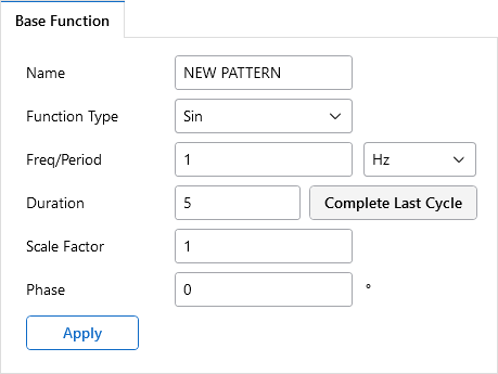
Time History Function: Base Function - tab Settings

Setting	Description
Function Type	Function Type allows you to define the type of function. Currently, a generated function may be defined as either a sine or cosine. Sin - Sine Cos - Cosine
Freq / Period	Freq / Period allows you to enter the function based on whatever criteria (Hertz, Rotations per Minute, or natural period) is most convenient for them. First choose the criteria, then enter the frequency / period. Criteria options are: Hz - Hertz RPM - rotations per Minute sec - (Seconds) the natural period of time
Duration (sec)	Duration allows you to change the length (in seconds) of the Time History function cycle.
Complete Last Cycle	The Complete Last Cycle button allows you to change the duration of the function so that the last cycle is completed.
Scale Factor	Scale Factor allows you to scale a function up or down by a given amount. This is often entered in as the total force produced by the sinusoidal function.
Phase (deg)	Phase allows you to identify the sinusoidal loading angle (in degrees) that starts at values other than the maximum or zero.
Apply	The ‘Apply’ button forces the plotted image of the function to be updated. The text of this button turns bold when the program detects that changes have been made that are not reflected in the current function plot.

Display Range

This section controls the display of the function. This may be useful when it is necessary to zoom in on certain times within the overall pattern / function, especially ramp up or coast down regions. This allows you to verify that the function is created correctly and that no discontinuity exists at the ramp up or ramp down transition points.

Time History Function: Display Range Settings

Setting	Description
Steps	The number of steps is not as relevant to generated functions because these are displaying general functions. The default displayed step is 0.001 seconds in the generation window and currently cannot be changed.
Apply	The ‘Apply’ button (found under the Base function section) forces the plotted image of the function to be updated. The text of this button turns bold when the program detects that changes have been made that are not reflected in the current function plot.

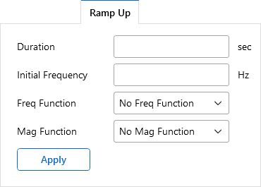
Ramp Up - tab

The Ramp Up tab controls how the frequency and magnitude change with time at the beginning of the function. When AutoCalc option is selected for the magnitude that means that it will vary with the square of the frequency. This can be thought of as the behavior of the equipment when it is first turned on before it attains its normal operating speed.

Time History Function: Ramp Up Settings

Setting	Description
Freq Function	The Frequency Function option lets you choose which frequency function to use for Ramp Up. Choices are; no Frequency Function, Linear Frequency Function or Quadratic Frequency Function.
Mag Function	The Mag Function option lets you choose which mag function to use for Ramp Up. choices are; no Mag Function, AutoCalc Mag Function, Linear Mag Function or Quadratic mag Function.
Apply	The Appl’ button forces the plotted image of the function to be updated. The text of this button turns bold when the program detects that changes have been made that are not reflected in the current function plot.

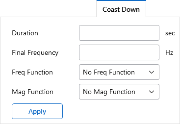
Coast Down - tab

The Coast Down tab controls the frequency and magnitude change with time at the end of the function. When AutoCalc option is selected for the magnitude that means that it will vary with the square of the frequency. This can be thought of as the behavior of the equipment as it is turned off and slows down from its operating speed.

Time History Function: Coast Down - tab Settings

Setting	Description
Freq Function	The Frequency Function option lets you choose which frequency function to use for Coast Down. Choices are; no Frequency Function, Linear Frequency Function or Quadratic Frequency Function.
Mag Function	The Mag Function option lets you choose which mag function to use for Coast Down. choices are; no Mag Function, AutoCalc Mag Function, Linear Mag Function or Quadratic mag Function.
Apply	The Appl’ button forces the plotted image of the function to be updated. The text of this button turns bold when the program detects that changes have been made that are not reflected in the current function plot.

Import Load

For more complex functions, the program allows importing from a text file. That text file must be written in a particular format in order to be read properly. See information below for a brief example:

[TIME_HISTORY_INPUT_DATA]

[HEADER]

Original Blast

[END_HEADER]

[FUNCTION_INFO]

[.MULTIPLIER] <1>

1 ;

[.END_MULTIPLIER]

[.TIME_STEP] <1>

0.1 ;

[.END_TIME_STEP]

[.RECORD_PER_LINE] <1>

1;

[.END_RECORD_PER_LINE]

[END_FUNCTION_INFO]

[RECORDS] <7>

0.

5.

3.

1.

-1.

-0.5

0.

[END_RECORDS]

[END_FILE]

The following table describes the main sections for the text file import.

Text File Import Main Sections

Section	Description
[HEADER]	The [HEADER] section is the name of the time history as it will appear in the library of time history patterns / functions. This section is a required field.
[FUNCTION_INFO]	The [FUNCTION_INFO] section gives information on the function itself, like time step, number of records per line, et cetera.
[.MULTIPLIER]	The [.MULTIPLIER] is used for converting the units of the record data. For example, acceleration records in RISA are assumed to be entered in terms of acceleration of gravity. If the record gives the acceleration in terms of meters per second squared, then this multiplier would be set to 0.10194 (1/9.81). This value will be assumed to be equal to 1.0 if not specifically entered.
[.TIME_STEP]	The [.TIME_STEP] is assumed to be 0.01 sec, if not entered.
[.RECORD_PER_LINE]	The [.RECORD_PER_LINE] field corresponds to the number of records per line. This will be assumed to be 1 if not entered. Note: Acceleration based functions are assumed to already be entered in terms of the acceleration of gravity (g). Therefore, it is not necessary to multiply. Text files which illustrate example functions exist in the RISA\Time History\ sub-folder of the main RISA directory. These are merely ASCII text files with an extension of *.TH to identify them as Time History functions.
[RECORDS]	The [RECORDS] section gives the actual time history records. These values may be separated by spaces, semi-colons or carriage returns. The <number> which follows this entry is the number of lines of data, not the total number of records. Therefore, if the file contains 3 records per line and 500 lines of data. This entry would say <500> not <1500>.

View / Edit

The View / Edit Time History Function window looks different depending on what type of time history function is being viewed. When it is a generated sinusoidal function, there are controls that allow the user to edit the function. This editing is performed with the same controls (Freq/Period, Ramp Up, Coast Down) shown in the Generate screen.

When it is an imported time history, the only editing that can be done is to shorten the duration time of the motion. This can be done, for example, if the imported Seismic Record contains 50+ seconds of data, but the strong motion data lasts only a fraction of that time. If this is desired, then enter cutoff time in the duration and the time history function will be truncated at that time.

Click on image to enlarge it

In this view / edit window, the Values table lists the time / value pairs for the function. This can be used to view the exact time at which the function reaches a maximum or the exact value of a function at a given moment in time.

Hovering the cursor over the graph makes a vertical gray line appear that follows the cursor, so long as it is hovered over the graph area. Clicking anywhere in the graph area highlights the corresponding values in the Values table on the right-hand side.

Time History Loads Spreadsheet

The Time History Loads spreadsheet allows you to assign one of the existing time history to specific nodes or all nodes in the model.

To access the Time History Loads spreadsheet:

1. Click on Time History Loads in the Explorer panel to the right side of the model editing panel.

   

   Click on image to enlarge it

   Alternatively, you can access the spreadsheet from the Spreadsheets ribbon.

   To access from the Spreadsheets ribbon

   1. Go to the Spreadsheets ribbon.

      

      Click on image to enlarge it

   2. Click the Data Entry icon.

   3. Click the Time History Loads checkbox.

   The Time History Loads spreadsheet opens.

   

   Click on image to enlarge it

   The following table provides information about the data in the Time History Loads spreadsheet.

   Time History Spreadsheet Columns

   Column	Description
   Tag	Each Time History Load definitions is automatically assigned a “Tag” (such as T1, T2, et cetera) as shown on the left side of the spreadsheet. These tags are assigned by the program and may not be edited. Time History Loads are included in the analysis by referencing this Tag in the Load Combinations spreadsheet. Multiple loads or lines of data may be assigned within a given time history tag.
   Label	A tab’s Label is editable and is used for your reference as an identifier for that specific set of time history loads. Only one label is allowed per time history tag, even if the tag contains multiple lines of data.
   Time Step (sec)	Time Step is used to specify the integration time step used in the time history analysis. Refer to the section titled What integration time step should I use? for more information on this subject. Only one time step is allowed for a given time history tag, even if the tag contains multiple lines of data. Note: You have the option of leaving the time step blank. If this is done the program automatically uses a value of 1/10th the lowest mode with at least 10% mass participation. If the time history forcing function were imported, the time step is not taken greater than the time step specified in the imported function. If your input time step is greater than either of the two above limits, a warning log message is produced. Using the HHT method for a Direct Integration solution in combination with a negative alpha integration constant, creates some energy dissipation of higher frequency response. This may allow you to set integration time steps that are greater than the values described above. If multiple Time Histories are applied at the same time for a single load combination, the lowest integration time step is used. If multiple time histories are applied to a load combinations, which do not overlap, each time history is integrated based on the smaller time step.
   Type	Type indicates whether this time history function applied to the model is a Force or an Acceleration. Units for each are reported in the status bar at the bottom of the application. Acceleration functions are always assumed to be given as a fraction of the acceleration of gravity.
   Function	Function identifies the Time History Function / Pattern that will be applied to the model.
   Node	Node indicates whether the time history load function is applied to the node specified. For seismic time history analysis, the node should be identified as ALL to indicate that the acceleration load is applied to the entire model.
   Dir	Dir (Direction Setting) identifies the direction of the load. This is input with respect to the global axes, X, Y, and Z.
   F Factor	F Factor is a magnification factor applied to the function. This can be used for any purpose you want. A common use would be to use F Factor to account for an increase in the operating speed of dynamic equipment, or to account for tributary area for a blast analysis. A blank value defaults to 1.0. For example, the BLASTLOADEXAMPLE function is really a time dependent pressure resulting from some form of explosion. The load is applied to individual joints thus the F Factor is used to enter the tributary area for each node. Therefore, this effectively converts the blast load from pressure to force. Click on image to enlarge it
   T Factor	T Factor adjusts the time steps in the forcing speed of the forcing function. A factor less than 1 increases the speed of the equipment and a factor greater than 1 decreases the speed of the equipment. This can be a quick and useful way to adjust a given TH function for variations in speed instead of having to create new functions for each case. A blank value defaults to 1.0. Click on image to enlarge it For example, the 0.9 T Factor is used to adjust the 3000 RPM function to something that is about 11% higher (1/0.9 = 1.11111). This would be about 3333 RPM. Similarly, use a factor of 1.10 is used to adjust the 3000 RPM function to something that is about 9% lower (1/1.10 = 0.90909). This would be about 2727 RPM. Note: One important consideration is that the integration time step is not automatically converted based on the T Factor. This is the reason the time step changes from 0.001 seconds to 0.00909 in the example above. This is only necessary in this example because the intent was to have exactly 20 integration steps for each full cycle of the sine wave. This means that there is an integration time step for every pi/10 radians of cyclic motion.
   Arrival (sec)	Arrival indicates the time at which the forcing function starts. A blank value defaults to 0.
   Run Out (sec)	Run Out indicates how long to continue the time history integration after the function has ended. A blank value defaults to 0.

2. (Optional) To include Time History Loads in the analysis, reference the load’s Tag in the ‘Load Combinations’ spreadsheet (as shown in the following example image).

   

   Click on image to enlarge it

What Integration Time Step Should I Use?

The answer to this question is a matter of engineering judgment, of course. And, a good reference on dynamic analysis should be consulted. However, there a few basic factors that come into play. This section is not meant to provide definitive recommendations on what the engineer should do. Rather it is meant to identify some common practices.

For dynamic equipment with a known excitation frequency, the answer is usually based on the operating frequency. A common choice would be to pick an integration step equal to 1/20th or 1/24th the operating period of the equipment. Though the exact fraction of the operating period can be debated, the 1/20th and 1/24th values ensure there is an integration step for every 18 or 15 degrees of rotation.

For a more random excitation (like seismic loading), the important consideration is more likely to be related to the natural frequencies of the structure which have significant mass participation. A common choice would be to make sure that the integration step is less than 1/10th the smallest significant natural period. Though again, the exact fraction of the significant period can be debated. It may also be necessary, however, to identify the frequency content of the forcing function and use a time step (similar to the 1/20th of the lowest equipment period) that can capture the frequency content of the forcing function.

Apply a Time History Load

To apply a Time History Load:

1. Click on Time History Loads in the Explorer panel to the right side of the model editing panel.

   

   Click on image to enlarge it

   Alternatively, you can access the spreadsheet from the Spreadsheets ribbon.

   To access from the Spreadsheets ribbon

   1. Go to the Spreadsheets ribbon.

      

      Click on image to enlarge it

   2. Click the Data Entry icon.

   3. Click the Time History Loads checkbox.

   The Time History Load spreadsheet opens.

   

   Click on image to enlarge it

2. Click in the Function column, then click the down-arrow and specify a function / pattern (as shown in the following image).

   

   Click on image to enlarge it

3. In the Time Step (sec) column, specify the time (in seconds) between each integration time step.
4. Use the Type column to indicate whether the entry corresponds to a force / moment or an acceleration.
5. Specify the node and direction using the Nodes and Dir fields.

6. The remaining columns adjust the force factor, the time step / period of the input motion and arrival time. These may be left blank if no modification is necessary.

   Note: If the load is to apply to all nodes in the model, enter the ‘Node’ label as "ALL".

Include a Time History Load in a Load Combination

To include a Time History Load in a Load Combination analysis:

1. Click on the BLC column of the Time History Load you want to include.

2. In the BLC column, type the Time History load Tag (T1, T2, etc.) into the cell.

   Alternatively, you can click the ellipsis button to open the Set Basic Load Combination Entry window where you can choose the appropriate Time History load from a drop down list, as shown in the following image.

   

   Click on image to enlarge it

3. In the Factor column, type in a corresponding BLC factor.

Required Number of Modes

The time history solution requires the use of the structure's mass matrix. In order to ensure that this matrix is present and valid, RISA requires an active Dynamic / eigen solution before a Time History Analysis can be run. The number of modes that need to be solved, however, depends on the Time History Solution method you choose.

Modal Superposition

For dynamic equipment with a known excitation frequency, the required number of modes is usually related to the operating frequency of the equipment. This means solving for all modes within certain percentage of the operating frequency of the equipment, even if those modes have little mass participation.

For more random excitation (like seismic loading), the important consideration is likely the total mass participation for the solved modes.

Direct Integration

The number of modes solved during a dynamic analysis does NOT affect the accuracy of the Time History solution when the Direct Integration solution method is chosen. The dynamic analysis is only required to ensure that RISA has a valid stiffness matrix available to be used during the time history solution.

Damping

Modal Superposition

When the Modal Superposition option is chosen, RISA requires you to enter in a single damping value which applies to all modes. While it is technically possible to assign a different damping value for specific modes, RISA does not currently support this behavior.

The modal superposition method does not support the building of a damping matrix. Therefore, your defined damping values, that are associated with translational or rotational springs, are not used in the solution.

Direct Integration

When the Direct Integration solution option is chosen, the damping matrix is generally built using the classic Rayleigh Damping formulation based on the Mass proportional and Stiffness proportional damping, as shown in the following equations where mu and kappa are merely constants used to form the damping matrix out of the existing mass and stiffness matrices.

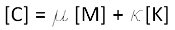
The relationships between mass and stiffness and frequency means that the % damping values vary with frequency (see curve below). These values can be adjusted so that a targeted damping ratio is achieved at two specific frequencies. In the image below, the target damping ratio was 5% at 15 Hz and 18.33 Hz. It remains relatively close to 5% between those target frequencies, but will be slightly less than 5%.

Click on image to enlarge it

You can directly assign the mu and kappa constants, or you can choose to use the window below, which is activated by clicking on the ellipsis button in the advanced solution window of the Model Settings. You need only enter in your targeted damping ratio and the two target frequencies, then the program will calculate a mu and kappa value that produces the desired damping for those frequencies.

Click on image to enlarge it

User Defined Spring Damping

When the structure is supported on spring boundary conditions, you can directly enter damping values using the boundary conditions spreadsheet or window. This directly sets the values of the damping matrix for those boundary condition degrees of freedom. The most common usage for this is when you want to use Rayleigh Damping for the super structure, but a higher damping ratio to model that represents the higher levels of damping that occur at the soil / structure interface, due to the radiation of the vibrational energy into semi-infinite material that is not part of the structural model.

Soil Properties

For industrial foundations subject to large dynamic forces, one of the variable properties to be considered are the properties (stiffness and damping) of the soil. This section is not meant to provide true recommendations on what the engineer should do. Rather it is meant to identify some common practices and point to some references which may discuss the matter in more depth.

Stiffness and Damping

One of the considerations for soil stiffness is the magnitude of the anticipated response. For most dynamic equipment, the amplitude of the vibration response may be assumed to be low. The type of elastic soil stiffness that is estimated in a soils report, may be intended to limit settlement or prevent soil failure. If so, this would be an inappropriately low estimate for a vibration response. That's because it is based on large strains at ultimate failure levels. Instead, it would be more appropriate to use a higher soil stiffness based on low magnitudes of vibration that are expected during normal operation.

The American Concrete Institute (ACI) has an excellent report titled ACI 351.3-R Foundations for Dynamic Equipment. This document references a number of other good technical sources. But, in the opinion of the Engineers at RISA, this ACI document is probably the best starting point for understanding how to set these parameters. In particular this document describes two common methods for assessing the stiffness properties of the soil.

Richart - Whitman Model: This is a frequency independent method of determining foundation stiffness (vertical, horizontal, and rocking) and damping. Equations for calculating this stiffness are found in section 4.2.1.1 of ACI 351.3-R.

Veletsos Model:This is a frequency dependent criteria for establishing soil stiffness (vertical, horizontal and rocking) and damping. The dominant operating frequency of the equipment would be the normal choice for calculating the Veletsos stiffness and damping values.

Unfortunately, it is not as simple as just calculating a value from these models and using that value. The final decision involves some engineering judgment and experience. Decisions which require engineering judgment:

• What criteria should be used for establishing the soil properties the Richard-Whitman (frequency independent) or the Veletsos (frequency dependent) model?
• How much variation should be assumed in the soil stiffness? Since the soil properties are not know precisely, do you run a separate analysis at +10% and -10% of the base values calculated?
• How do you adjust the damping values? The ACI sections referenced above describe the radiation / geometric damping that would occur. This likely accounts for the majority of the energy loss in the soil, but there is also material damping (somewhere between 2 and 5% of critical damping) that would occur as well.
• What is the maximum damping value allowed per your design criteria? There is often design criteria that will limit the maximum damping to be considered in the analysis to some percentage of critical damping.

Results - Time History Trace

When Time History results are available, you can view a trace of particular node results as a function of time.

To view Time History Trace Results:

1. Go to the Results ribbon.

   

   Click on image to enlarge it

2. Click on the TH Trace icon in the Time History section.

3. In the model, click on the Node you want to see the Time History results for.

   In the following example, we chose N31.

   

   Click on image to enlarge it

4. (Optional) Click on the Values to Trace down-arrow and choose the values you want to view.

   Options are Displacement, Velocity, Acceleration or Reaction.

5. (Optional) Click on the second block down-arrow (as shown in the following image) to choose a different axis direction to view.

   

   Click on image to enlarge it

   You can display as the X, Y or Z direction. Though, you can also choose to view the RX, RY or RZ rotational displacement, velocity, acceleration or moment reaction. These values are all given with respect to the global axes.

6. (Optional) Use the Display Range section to view only selected portions of the solved data, if extra clarity is needed for a relative tight window of time. Make sure you ‘Apply’ your selection for the view to change accordingly.

   

   Click on image to enlarge it

7. (Optional) Click the Print button to open the Print Options window.

   The Print Options window allows you to print the trace as an image. Several formats may be listed, depending on the programs you have installed on your PC.

   You can also export the data to an ASCII text file that can be opened in Excel or Access. See Export Time History Traces for instructions.

Results - Export Time History Traces

The Export TH Trace feature allows you to export a series of time history traces to an ASCII text file that can be opened in Excel. This can be done for a graphical selection of nodes.

To export a Time History Trace:

1. Go to the Results ribbon.

   

   Click on image to enlarge it

2. Click on the Export TH Trace icon in the Time History section.

   This icon becomes available whenever a valid time history solution is present.

   The Batch Export Time History Traces window opens.

   

   Click on image to enlarge it

   The following table provides descriptions for the sections in this window.

   Batch Export Time History Traces

   Section	Description
   Values to Export	The ‘Values to Export’ section allows you to choose whether to export displacements, velocities, accelerations, reactions or input functions. It also lets you dictate which direction the export is being performed on.
   Field Delimiter	The ‘Field Delimiter’ section allows you to choose what characters are used to separate individual fields.
   Load Combinations	The ‘Load Combinations’ section allows you to export for all the solved time history load combinations or only a single one. It also allows you to export only a specific time range of the overall response. This allows you to ensure that you are getting only the steady response when performing an equipment vibration analysis and that any transient response, due to start-up effects, can be excluded.
   Report Section Options	The ‘Report Section Options’ allows you to control the column headers in the ASCII text files, as well as whether or not you want to see the time values or time steps in the file itself.

3. Choose all the options that correspond to the data you want exported.

4. Click the Export button.

Results - Animate Time History Deflection

When a time history load combination has been solved, you can build a animation movie of the deflected shape of the structure as a function of time. You can speed up or slow down the animation to control the length of the movie, and you can pause it and re-start it at a particular time step or time.

View a Time History Animation

To view a Time History animation:

1. Go to the View ribbon.

2. Click the Results icon in the ‘Animate’ section.

   An Animation Settings window opens.

   

   Click on image to enlarge it

3. Click on the Time History option.
4. Click the Load Combination down-arrow and select the load combination you would like to animate.
5. Click on .

   The Animation window opens displaying am animation similar to what is shown here:

   

   Click on image to enlarge it

Add Trace Data to the Animation

To add Trace Data to the animation:

1. Click the Trace icon.

   A Set Trace Reference window opens.

   

   Click on image to enlarge it

2. Click on the node Direction you want to specify (X, Y or Z, or X Rot, Y Rot or Z Rot. Note that ‘Rot’ = rotation).
3. Click on the Display Type (Displacement, Reaction or Input Function).

4. Click OK.

   A Time History Trace of the specified joint result or input function is appended to the bottom of the deflection animation, as shown in the following image.

   

   Click on image to enlarge it

Member Stiffness Issues

Cracking for Concrete Member

The Design tab of the Load Combinations spreadsheet has a ‘Service’ checkbox which indicates whether the loading is at service level or ultimate level.

Click on image to enlarge it

Service - checked: If the Service checkbox is checked, the concrete stiffness will be the larger stiffness assumed for service level loads.

Service - unchecked: If the Service checkbox is unchecked, the concrete members will have the lower stiffness that is applicable for ultimate level loads.

What Solution Method should I Use?

Two different Time History procedures are discussed in detail in the Solution topic.

The choice between the two solution methods comes down to questions about solution speed and damping. The ‘Modal Superposition’ method is faster for models that don't require large number of modes in the dynamic solution. But, the advantage in solution speed gets reduced as the number of modes solved gets very high. Therefore, this solution method would normally be used in cases where solution speed is the main consideration.

The ‘Direct integration’ procedure doesn't technically require any modes to be solved. However, RISA requires that one mode be solved so that the program can build and validate the mass matrix before the Time History solution. Therefore, in models where it is very difficult to capture enough modes to get a comfortable level of mass participation, the Direct Integration procedure would likely be chosen. In addition, the Direct Integration method allows you to directly set damping values at boundary condition springs. Therefore, in models where this extra sophistication in the damping terms is required, the Direct Integration method is the obvious choice.